Adding new meshing domains
As explained in chapter FIXME Nadamak provides meshing capabilities interfacing GMSH via data files produced from pre-defined templates. The template files describe parameterized geometric models. When mesh is generated the parameters are substituted in Matlab producing input files for GMSH. The generated mesh is read back from mesh file and presented to user as a Mesh object.
The whole machinery of templates handling and calling GMSH is hidden behind convenient object oriented interface described in section FIXME. Here we take a closer look at this machinery by following a step by step explanation how a new geometric model can be added to Nadamak. The steps involve:
- Creation of non-templatized geometric model for GMSH.
- Implementation of a class derived from mp.Geom to wrap the geometric model.
- Templatization of GMSH input file and linking it with Matlab class.
- Introduction of more advanced features as subdomain and meshing control variables.
These steps will be illustrated in details on the example of geometric model of a quarter of notched rectangle domain shown in Fig. 1.
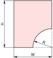
Fig. 1 Geometric domain of a quarter of notched rectangle.
Creating GMSH geometry input file
The starting point in adding new meshing domain is to prepare a valid GMSH geometry file describing the desired geometry. This file will will be then turned into template file processed by Matlab, but first one has to make sure that there is no error in geometry definition and GMSH is able to produce a mesh from this file.
To complete this step some knowledge of GMSH scripting language is required. In GMSH geometries are described using boundary representation (B-Rep). The model is built by successively defining primitives of increased complexity and dimension, starting from points, curves, surface and volumes.
When looking at Fig. 1 we can see that it is parameterised by three parameters \(W,H\) and \(R\). It is advantageous to introduce these parameters right from the start in the GMSH geometry file, for the moment giving them some fixed value. When creating B-Rep representation of our geometry we should already envisage how it should be decomposed into geometric elements in order to make convenient application of attributes such as boundary conditions, loads or material properties. Having this in mind the arc is split into two pieces by a point \((x_a, y_a)\). To make this splitting flexible we introduce additional parameter \(t \in [0, 1]\) that describes the position of the point on arc via formula
The complete GMSH input file is shown in listing Listing 1. Additional parameter \(lc\), defined in the first line, is the desired edge length of the generated mesh in the neighbourhood of the given point.
IMPORTANT The interface to GMSH implemented in Nadamak assumes that in the
generated mesh at least one physical region is present. Thus, while it is not strictly
necessary for running GMSH, in the last line in Listing 1
a region with name d_whole is defined. The names assigned to regions are arbitrary
as long as they can be used as Matlab variable names.
lc = 0.5;
R = 1;
W = 2;
H = 3;
t = 0.5;
xa = W-R*Cos(t*Pi/2);
ya = R*Sin(t*Pi/2);
Point(1) = {0,     0, 0, lc};
Point(2) = {W-R,   0, 0, lc};
Point(3) = {xa,   ya, 0, lc};
Point(4) = {W,     R, 0, lc};
Point(5) = {W,     H, 0, lc};
Point(6) = {0,     H, 0, lc};
Point(7) = {W, 0, 0};
Line(1) = {1,2} ;
Circle(2) = {2,7,3};
Circle(3) = {3,7,4};
Line(4) = {4,5};
Line(5) = {5,6};
Line(6) = {6,1};
Line Loop(1) = {1, 2, 3, 4, 5, 6};
Plane Surface(1) = {1};
Physical Surface("d_whole") = {1};
Having the file defined we can load it into GMSH to check if the geometry is defined properly as illustrated in Fig. 2.
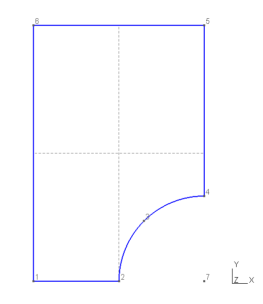
Fig. 2 GMSH visualisation of geometry defined in Listing 1.
The last step is to run GMSH to generate mesh for the defined geometry as illustrated in Fig. 3.
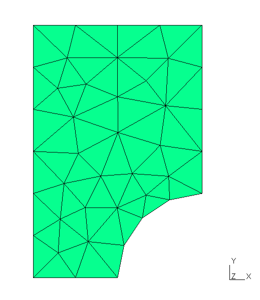
Fig. 3 Mesh generated from the file shown in Listing 1.
Creating geometry template file
Having GMSH input file properly defined we can not turn it into geometry
template file. We just need to copy the file into specific folder and change
its extension to :code`*.tpl`. In Nadamak all geometry template files are store
in folder mesher/gmsh/geomodels. For the subsequent steps we assume that
the code in Listing 1 is saved in file
mesher/gmsh/geomodels/notchedrectquarter.tpl.
Defining Matlab class for geometric model
To nicely handle geometric domain defined in notchedrectquarter.lst we need
to define a class derived from mp.GeomModel. The base class
mp.GeomModel provides functionality common to all geometric domains.
It also defines interface than each specific geometry class must obey to
smoothly integrate with the rest of Nadamak package. Here we assume that our
class will be called NotchedRQGeom [1]. The definition of this class
shown in Listing 2 is put in file
package/+mp/+geoms/NotchedRQGeom.m alongside other geometric domain
classes.
1 2 3 4 5 6 7 8 9 10 11 12 13 14 15 16 17 18 19 20 21 22 23 24 25 26 27 28 29 30 31 32 33 | classdef NotchedRQGeom < mp.GeomModel
% Geometric model for a quarter of notched rectangle.
properties (Access=public)
params = struct();
end
methods(Access=private)
function setup(obj, params_)
end
end
methods
function [obj] = NotchedRQGeom(name, params, legacyID)
if nargin < 3
legacyID = 810;
end
if nargin < 2
params = struct();
end
obj = obj@mp.GeomModel(name, 2, legacyID);
if ~isempty(params)
obj.setup(params);
end
end
function [regionNames] = regions(obj)
regionNames = {'d_whole'};
end
function [name] = templateName(obj)
name = 'notchedrectquarter.tpl';
end
function [maxlc] = coarsest_lc(obj)
maxlc = 1;
end
end
end
|
Lines 11-22 define NotchedRQGeom constructor. The constructors for
geometric domain classes look virtually the same. The real work to construct an
object is delegated to setup method defined at lines 7-8. For a moment
setup method is empty, but later we extend it when adding more
functionality to our class. The legacyID variable define in line 13 is
the reminiscence of the old design in which each distinct geometric model had
unique numeric ID. The value assigned to legacyID is arbitrary with one
condition that it should be greater than 100.
Attention should be paid to line 18. At this line the constructor of base class
is called. The second argument of mp.GeomModel constructor is the
geometric dimension of the model. All geometric models are embedded in
3-dimensional real space, but themselves they can be 1D, 2D or 3D objects.
As our NotchedRQGeom class is derived from mp.GeomModel
abstract base class it has to define the following three methods
regions(obj)- method that return names of physical regions as a cell array of strings.templateName(obj)- method that returns the name of geometry template file.coarsest_lc(obj)- method that return the real value used as mesh density parameter. Nadamak provides some convenience functions to visualize geometric domains but this can be done only via meshes generated on them. The mesh density parameter returned bycoarsest_lcmethod is just an educated guess about mesh density that will still capture geometric features of the domain but the same time will have the smallest number of elements to not induce unnecessary overhead.
Having NotchedRQGeom class defined we can use it in the meshing
framework. The example shown in Listing 3 produces mesh
shown in Fig. 4.
1 2 3 4 5 6 7 8 | mesher = mp.Mesher();
geom = mp.geoms.NotchedRQGeom('my_domain');
mesh = mesher.generate(geom, struct('lc', 0.8));
viewer = mp.Viewer();
viewer.show(mesh);
|
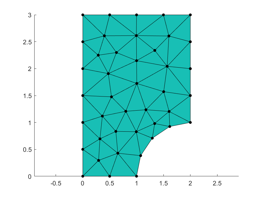
Fig. 4 Mesh generated and visualized in Listing 3.
Extending NotchedRQGeom class
At this moment we can notice that the class NotchedRQGeom is sort of
a dumb one. We can use it to generated mesh in the specific geometry, but we
have no means of controlling the model dimensions nor meshing parameters. This
is related to the fact that the geometry template file
notchedrectquarter.lst is all the time the same, thus GMSH produces all the
time the same mesh.
The first step in adding features to NotchedRQGeom is to turn
notchedrectquarter.lst into true template file as shown in
Listing 4. In highlighted lines instead of specific
values we put named placeholders obeying the syntax < name >. The
placeholder name can be arbitrary as long as it is a valid Matlab identifier
[2].
lc = <lc>;
R = <dR>;
W = <dW>;
H = <dH>;
t = <amid>;
xa = W-R*Cos(t*Pi/2);
ya = R*Sin(t*Pi/2);
Point(1) = {0,     0, 0, lc};
Point(2) = {W-R,   0, 0, lc};
Point(3) = {xa,   ya, 0, lc};
Point(4) = {W,     R, 0, lc};
Point(5) = {W,     H, 0, lc};
Point(6) = {0,     H, 0, lc};
Point(7) = {W, 0, 0};
Line(1) = {1,2} ;
Circle(2) = {2,7,3};
Circle(3) = {3,7,4};
Line(4) = {4,5};
Line(5) = {5,6};
Line(6) = {6,1};
Line Loop(1) = {1, 2, 3, 4, 5, 6};
Plane Surface(1) = {1};
Physical Surface("d_whole") = {1};
The second step is to modify definition of NotchedRQGeom class by
defining parameters corresponding to placeholders in geometry template file and
respectively fixing setup method to properly initialize the parameters
either form constructor arguments or from default values. New version of
NotchedRQGeom class is shown in Listing 5 with new
lines highlighted.
classdef NotchedRQGeom < mp.GeomModel
  % Geometric model for a quarter of notched rectangle.
  properties (Access=public)
    params = struct('dW', 2, 'dH', 3, 'dR', 1, 'amid', 0.5);
  end
  methods(Access=private)
    function setup(obj, params_)
      obj.params.dW = mp_get_option(params_, 'dW', obj.params.dW);
      obj.params.dH = mp_get_option(params_, 'dH', obj.params.dH);
      obj.params.dR = mp_get_option(params_, 'dR', obj.params.dR);
      obj.params.amid = mp_get_option(params_, 'amid', obj.params.amid);
    end
  end
end
With geometry template file and the class augmented in the above way it is now possible to control both geometry and mesh density as shown in Listing 6.
1 2 3 4 5 6 7 8 9 10 | mesher = mp.Mesher();
geom = mp.geoms.NotchedRQGeom('my_domain');
geom.params.dR = 0.5;
geom.params.dH = 1;
mesh = mesher.generate(geom, struct('lc', 0.1));
viewer = mp.Viewer();
viewer.show(mesh);
|
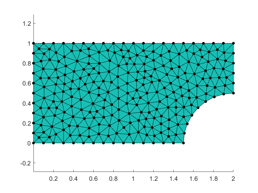
Fig. 5 Mesh generated and visualized in Listing 6.
The exercise of extending the class NotchedRQGeom clearly shows how
simple is the mechanism for passing data from Matlab level to GMSH. This
mechanism is based on textual substitution of placeholders in a template file
by values of corresponding Matlab variables. The substitution values come
either from geometric model object, for instance model dimensions, or form
mesher object, for instance mesh density parameters. The values passed passed
from Matlab to GMSH, can be either scalars or vectors. In case of vector valued
parameters the substitution string is formed by values of vector elements
separated by comas without any other syntactic characters. Thus to properly
handle such substitutions on GMSH side, one has to make sure that proper GMSH
syntax for list literals is used. This is illustrated in
Listing 7.
vecparam = {<vecparam>};
Similar rule applies to the case of string valued parameters. Further extensions to a geometric model class and template file are case specific and will strongly dependon functionality provided by GMSH scripting language. Below we discuss some extensions that are likely to be relevant to many geometric domains. They are:
- subdivision of domain into subdomains,
- selection of the type of generated elements,
- management of mesh density by local refinements,
- handling boundary regions,
- independent meshing of regions and their combinations.
Subdivision of meshing domain into subdomains
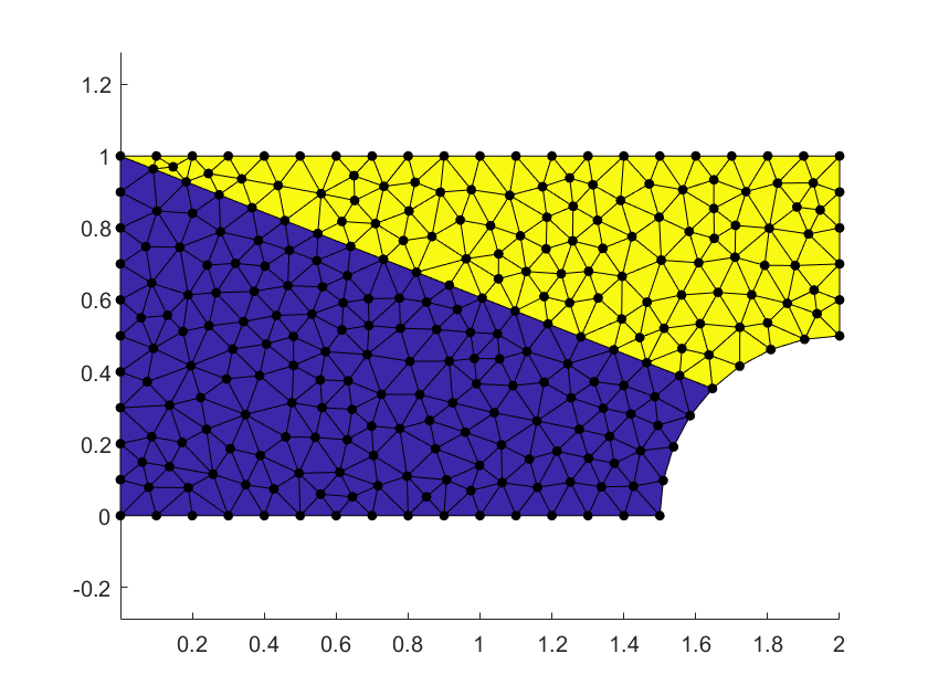
Fig. 6 Meshing domain subdivided into subdomain.
Footnotes
| [1] | While not strictly necessary the naming convention addopted in Nadamak is such that names of classes for geometric models have the Geom suffix. |
| [2] | While not strictly necessary the naming convention addopted in Nadamak is such that names of placeholders corresponding to dimension parameters have d prefix, for instance dL, dH, etc. |